Preliminary: LR and LL grammars
Read through parsing tbh.
§ 5. Syntax-directed translation
Chapter 5 deals with something called syntax-directed translation. The Dragon Book states:
Important
Syntax-directed translation is done by attaching rules or program fragments to productions in a grammar (52).
This sounds really complicated, but is actually really fuckin simple. Basically, let’s say you have a grammar for a language; in this case, we’ll do a simple infix math expr lang:
expr = expr + term
     | expr - term
     | term
term = 0 | 1 | ... | 9
Obviously, there are a few things you might want to do with an expression. In particular, you might perform a translation of this program from one form to another. For instance, you might want to turn this into a postfix program. Or, you might want to transform terms from integers to roman numerals. Or, you might want to do constant folding (which in this case, is just evaluation lmao). Translation is a generalization of “compilation,” which implies translating to machine code I guess. Basically, you want to compute some value based on the expression.
A syntax-directed translation is exactly what it sounds like: the syntax tree guides how this translations are executed. Basically, it’s any process where these translations are performed using rules/programs that are attached to BNF grammar rules.
So how are these translations notated and specified? There are two main ways of doing so:
- Syntax-directed definitions. For each BNF rule for a non-terminal, you define what the value of the translation—the attribute—should be for that non-terminal, in terms of the attributes of its children. For instance, the postfix translation of
expr + termshould beformat!("{}{}+", expr.t, term.t), where[thing].tis the attribute of[thing]. This is basically anegg::Analysis, a declarative way of specifying translations based on declarative rules for non-terminals’ attribute (i.e., translation) values. - Syntax-directed translation rules. Instead of specifying the translation value for a rule directly, at each rule, you can specify that at some point during parsing, you should call some code (a “program fragment”)! For example, you could say
expr + term {print('+')}, meaning: “parse the sub-tree ofexprandterm, then executeprint('+').” If you add that print after every rule, you’ll get postfix printed out!
These are compressed definitions, we’ll go over each in-depth below.
Syntax-directed definitions
Remember egg::Analysis? This was a way of attaching some value to every e-node by defining some program that operates on the analysis values of its children. This is an example of a constant-folding analysis:
fn make(egraph: &EGraph<SimpleMath, Self>, enode: &SimpleMath) -> Self::Data {
	let x = |i: &Id| egraph[*i].data;
	match enode {
		SimpleMath::Num(n) => Some(*n),
		SimpleMath::Add([a, b]) => Some(x(a)? + x(b)?),
		SimpleMath::Mul([a, b]) => Some(x(a)? * x(b)?),
		_ => None,
	}
}
This is basically what a syntax-directed definition is. For every rule for a non-terminal in our BNF, we define what the analysis—an attribute—of that non-terminal should be, in terms of the attributes of its children. In an SDD, every production has an associated semantic rule, dictating how that production rule should compute the attribute for that non-terminal. Let’s look at the semantic rules for a postfix translation of our math expr lang:
production                  semantic rules
---------------------------+-------------------------------------
expr = expr_1 + term        expr.t = expr_1.t || term.t || '+'
     | expr_1 - term        expr.t = expr_1.t || term.t || '-'
     | term                 expr.t = term.t
term = digit                term.t = digit.lexval
Pretty straightforward. For each production, we determine how the attribute should be calculated if that production applies. The translation is given by the attribute of the root note. It’s an egg::Analysis!
You can imagine that we’ve created a parse tree for this expression (like an e-graph), then attached an attribute at every node of this tree (like executing an Analysis). Translations don’t actually need to explicitly build this tree, but it’s helpful to visualize:
(4 + 2 - 5) expr.t = 42+5-
├── (4 + 2) expr.t = 42+
│   ├── 4 expr.t = 4
│      └── 4 term.t = 4
│   	    └── 4 digit.lexval = 4
│   └── 2 term.t = 2
│       └── 2 digit.lexval = 2
└── 5 term.t = 3
    └── 5 digit.lexval = 3
Some extra notes:
- We use dot notation to indicate attributes. In this case, we’ve named our attribute
t! - We denote
expr_1instead of justexprto separateexpr.tandexpr_1.t ||here is the string concat operator, following the Dragon Book’s lead.[thing].lexvaljust means whatever the value of the literal was.
Inherited and synthesized attributes
In this scheme, there are two kinds of attributes:
- Synthesized, which is all of what we just saw: we’re defining attributes for the parent (
expr_t) in terms of itself and its children (expr_1.t,term.t). - Inherited, which we haven’t seen yet, where we define the child in terms of its parent, itself, and its siblings.
- We don’t need to include “its children” in this defn, since we can recover that by adding
- Terminals can’t have inherited attributes, since that would mean the value of a terminal (e.g., a constant digit like
5) depends on the context in which it appears. This is why we have thelexvalstuff.
Inherited attributes are useful if your parse tree doesn’t “match” the AST of your source code. As an example, let’s look at this BNF for defining C-style typedefs:
T = B C
B = "int"
  | "float"
C = [<num>] C
  | ""
This is a right-recursive grammar! The parse tree for int[2][3] might look like:
T int[2][3]
+-- B int
\-- C [2][3]
    +-- [
    +-- <num> 2
    +-- ]
    \-- C [3]
        +-- [
        +-- <num> 3
        +-- ]
        \-- C ""
Note
In the book,
is the empty string ("").
We might want to translate this into an array type in the form: array(2, array(3, int)). But that tree structure differs greatly from our parsed tree structure; in particular, our type is the leaf at the very end!
We can use inherited attributes to pass information from one child to another child, allowing for communication between children:
production       semantic rules
----------------+------------------------------------------------
T = B C          T.t = C.t; C.b = B.t
B = "int"        B.t = int
  | "float"      B.t = float
C = [<num>] C_1  C.t = array(num.val, C_1.t); C_1.b = C.b
  | ""           C.t = C.b
Here, the inherited b attribute is propagated downwards all the way to the final leaf node of the C production, where it becomes the base case type value.
S- and L-attributed definitions
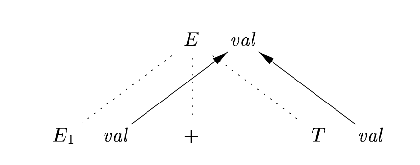
You can draw dependency graphs to determine which attributes depend on which other ones, like this one from (311):
Simple dep graph example
In some cases, attributes can be recursive and depend on each other infinitely. You can structure your SDDs
S-attributed definitions only consist of synthesized attributes. Thus, they can be evaluated bottom-up postorder (children left-to-right, then parent)
L-attributed definitions consist of synthesized attributes and inherited attributes where a child’s sibling attribute values (inherited or synthesized) are only depended on if they occur earlier in (i.e., to the Left of) the child node. Inherited attributes can also use inherited attributes of its parent, and other attributes of itself as long as they don’t cause cycles in the dep graph. This creates a consistent order that attributes can be evaluated in.
Evaluation order & side effects
An attribute grammar is an SDD without side effects. This subset of SDDs allow evaluation in any order that respects the dependency graph.
If you do have side effects, there are two options:
- Permit incidental side effects that don’t constrain/affect attribute eval (e.g., print logging)
- You can treat this as creating a new dummy synthesized attribute at the head of the production, where the rule is just calling the side effectful fn
- Constraint eval order so that same translation is produced for allowable orders (i.e., add implicit edges to the graph)
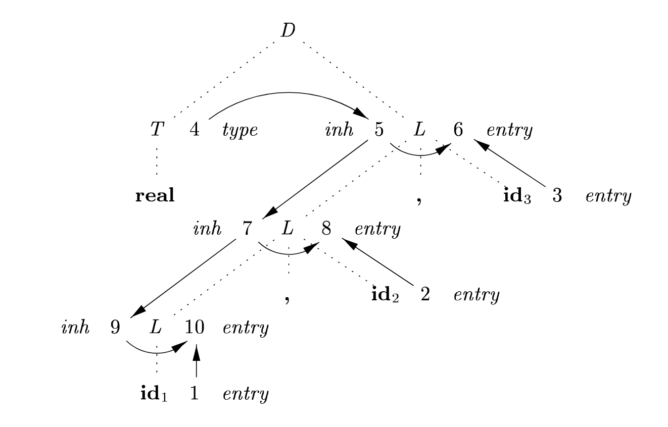
Complex dep graph example, w/ side effects
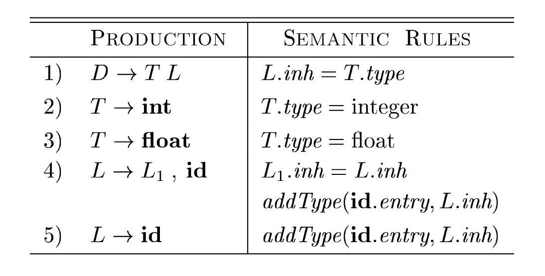
Given the following SDD:
The annotated parse tree for
float id_1, id_2, id_3:
The numbers are node IDs, 1-10. Nodes 1-3 are terminal
ids, which each have an attributeentry, which points to an interned string (i.e., symbol-table object).realshould befloat, that’s an error.
addTypeis a side effectful function that modifies the environment so thatidis recorded as having typetypein theinhattribute. This creates a new dependency.
Okay who cares
Most of the time you’re not constructing postfix strings, but more complex expressions. For instance, you might be building a syntax tree:
production                  semantic rules
---------------------------+-------------------------------------
expr = expr_1 + term        expr.n = BinOp "+" expr_1.n term.n
     | expr_1 - term        expr.n = BinOp "-" expr_1.n term.n
     | term                 expr.n = term.n
term = digit                term.n = Leaf digit digit.val
     | id                   term.n = Leaf id id.entry
You can also do this in L-attribute, LL, top-down style instead of S-attribute, LR, bottom-up style too. For instance, what if we parsed 2 + 4 as [2, + 4] instead of [2, 4]?
production                  semantic rules
---------------------------+---------------------------------------------------
E  = T E'                   E.n = E'.syn; E'.inh = T.n
E' = + T E_1'               E_1'.inh = Node "+" E'.inh, T.n; E'.syn = E_1'.syn
   | - T E_1'               E_1'.inh = Node "-" E'.inh, T.n; E'.syn = E_1'.syn
E' = ""                     E'.syn = E'.inh

T = (E)                     T.n = E.n
T = id                      T.n = Leaf id id.entry
T = num                     T.n = Leaf num num.val
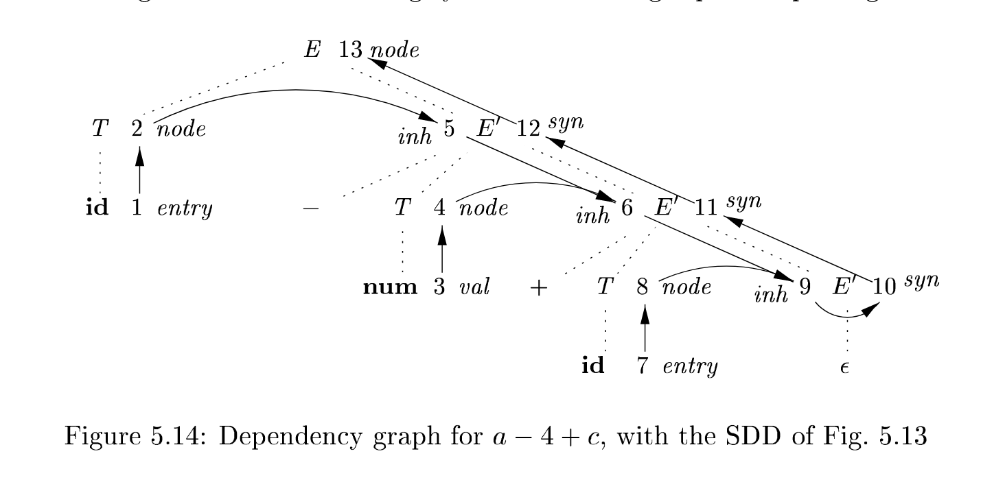
Here, we pass the left-hand arg as an inherited attribute into the child. At the leaf
Associated dep graph
Syntax-directed translation schemes
Where SDDs are a declarative way of specifying translations, syntax-directed translation schemes (SDTs) are an imperative way of specifying translations. They are equivalent in power to SDDs.
In a translation scheme, parse order in a production rule always goes left-to-right, depth-first. We can then intersperse a program fragment { <program> } wherever we want something to be executed. Here, we don’t conceptualize a translation as building a parse tree and assigning attributes to each node, but instead as executing instructions during parsing.
Converting LR S-attribute SDDs
We can trivially convert an S-attributed SDD into an SDT by just putting all of the actions at the end, in what’s called a postfix SDT:
expr = expr_1 + term { print("+") }
     | expr_1 - term { print("-") }
     | term
term = digit         { print(digit) }
Since we move left-to-right, depth-first, executing a print at the end of each rule means we’re basically doing postorder printing.
For constant folding, we can use these program fragments to store an attribute containing the value of the expr:
expr = expr_1 + term { expr.val = expr_1.val + term.val }
     | expr_1 - term { expr.val = expr_1.val - term.val }
     | term          { expr.val = term.val }
term = digit         { term.val = digit.lexval }
In an LR parser, since we have a stack of symbols already, we can keep track of attributes by just also keeping track of the attributes of each symbol along with the symbol itself in the stack.
Non-postfix SDTs
But actions don’t just have to be postfix! For a production B = X {a} Y, we execute {a}:
- As soon as
Xis at the top of the stack in LR parsing - Right before we attempt to expand
Yin LL parsing
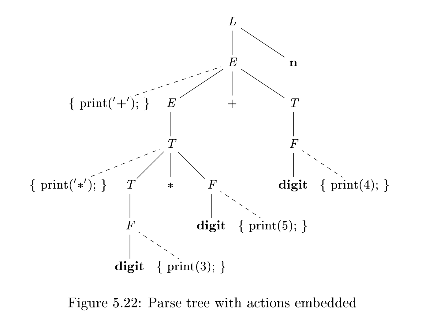
Not all of these non-postfix SDTs can be implemented during parsing. For instance, if you have a production rule:
E = { print('+') } E_1 + TYou can’t know + will happen and print that out before parsing it!
You can, however, implemented all SDTs if you assume a separate parse phase before applying actions:
- Build a parse tree, where all children are ordered left-to-right, including actions! (see example below)
- Preorder traverse, executing actions if visited
Parse tree with nodes
Eliminating left recursion
An LL (top-down) parser can’t deterministically parse a left-recursive grammar, since it can’t know when the left recursion will stop! We can transform left-recursive grammars into right-recursive ones like so:
A = A term1 | term2
(* into *)
A = term2 R
R = term1 R | ""
So term2 is now handled by term2 (R = ""), and repetitions of term1 are now handled by R, right-recursively. This encodes the intuition that A is defined by term2 and then a repetition of term1 0 or more times.
Note
See also Recursive rules.
Now let’s look at an example with SDTs:
E = E + T { print('+') }
  | T
Here, term1 = + T { print('+') }. Applying the transformation, we get:
E = T R
R = + T { print('+') } R
Notice how the action is in the middle!
Eliminating left recursion for S-attributed SDTs
If you’re assigning to attributes in your program fragments, we gotta get a little more specific. Let’s start with S-attributed SDTs first. Let’s go over this abstract example:
A = A_1 Y { A.a = g(A_1.a, Y.y) }
  | X {A.a = f(X.x) }
Let’s start the translation. We’ll do the first part of the translation, which encodes the intuition that A must start with X and then repeat 0 or more times:
A = X R
R = Y R_1 | ""
The general idea is that we propagate our accumulated attribute values top-down by setting an inherited attribute i. You can think of this as doing a foldl with an accumulator i. A, and thus R, needs access to X’s attribute value X.x to figure out this calculated value so far, so we assign that through an inherited attribute before parsing R.
A = X { R.i = f(X.x) } R
R = Y R_1 | ""
In the recursive case, we pass the accumulated attribute value as the inherited attribute of the recursive child.
A = X { R.i = f(X.x) } R
R = Y { R_1.i = g(R.i, Y.y) } R_1 | ""
In the base case, we set the actual attribute we care about to the inherited accumulator:
A = X { R.i = f(X.x) } R
R = Y { R_1.i = g(R.i, Y.y) } R_1 | "" { R.s = R.i }
And we do this in the other cases as well.
A = X { R.i = f(X.x) } R { A.a = R.s }
R = Y { R_1.i = g(R.i, Y.y) } R_1 { R.s = R_1.s } | "" { R.s = R.i }
If you’ll notice, this is basically what we did in Okay who cares when turning into non-left-recursive form!
SDTs for L-attributed definitions
For L-attributed definitions, translating an SDD into a SDT involves the following steps:
- Action(s) that compute an inherited attr for
Ashould be placed immediately beforeA, in dependency order. - Action(s) that compute synthesized attributes for the head of a production get put at the end.
§ 6.2.4. Single static assignment (SSA)
Single static assignment (SSA) form is a form of a program with two key attributes:
- Every variable is only defined once. No variable is redefined or shadowed or mutated, ever.
- Where two diverging control paths rejoin (e.g., after a branch), we use the
function to denote “pick the value based on which branch was taken.”
Example:
a = 2
b = 3
b = 4
if a > b:
	c = 9
else:
	c = 4
becomes
a1 = 2
b1 = 3
b2 = 4
if a1 > b2:
	c1 = 9
else:
	c2 = 4
c = phi(c1, c2)